
This is part 2 of a three-part series describing text processing and classification. Part 1 covers input data preparation and neural network construction, part 2 adds a variety of quality metrics, and part 3 visualizes the results.
Contents
In part 1 we did the bare minimum to create a functional text classifier. In the real world, we like have multiple indicators of performance. This post will demonstrate how to add more extensive measuring and logging to our model.
Full code described in this entry available on GitHub, in dbpedia_classify/tree/part2.
Prerequisites
Tensorflow (for real this time)
Sacred. Version 0.7b3 or greater; note that as of this writing the published version is 0.6.1. So install with
pip install sacred==0.7b3 |
Monitoring the Input Parameters
Every model has parameters. In addition, we often have training parameters (such as batch size) which may not be directly part of the model but are nonetheless important to record. When prototyping it’s convenient to just fiddle with the values and not necessarily store the results, but at some point it’s time to keep records. Sacred makes this reasonably easy.
First, we define an experiment object:
from sacred import Experiment from sacred.observers import FileStorageObserver ex = Experiment('my_runs', interactive=True) |
The ex object has to be declared before any of the decorators can be used.
To store parameters as part of a configuration, we define them in a function, and decorate that function:
@ex.config def default_config(): """Default configuration. Fixed (untrainable) word embeddings loaded from word2vec""" ## Parameters # Vocab Parameters max_vocab_size = 5000 min_word_count = 10 vocab_path = 'word2vec_vocab.p' # Network parameters embedding_size = 300 max_input_length = 500 # Training parameters batch_size = 100 batches_per_epoch = 10 epochs = 100 embedding_trainable = False build_own_vocab = False use_google_word2vec = True .... |
For alternate configurations, we can create a named config, and only overwrite the parameters we want to:
@ex.named_config def trainable_embed(): """ Load Google word2vec but allow it to be trained """ embedding_trainable = True build_own_vocab = False use_google_word2vec = True |
Note that the configs must be defined in the correct order, default in the beginning and overwrites happening later.
To make parameters available to a function, we “capture” that function:
@ex.capture def build_lstm_model(vocab_size, embedding_size, max_input_length, num_outputs=None, internal_lstm_size=100, embedding_matrix=None, embedding_trainable=True): ...function body here... |
Later on, we can run this function providing a few of the parameters:
The max_vocab_size, embedding_size, embedding_trainable, and max_input_length parameters are all provided by the config and not in the main body. There are two downsides to this, both are fairly minor
- Parameters must named the same thing in the function input and configuration, and so are effectively global. Since they are configuration parameters this makes sense. Occasionally I think the best name for a local scope isn’t the same as the global scope (e.g. witness
num_outputsandnum_classesabove) so that becomes tricky. - Providing some positional arguments looks super weird but apparently works. We provide
vocab_sizeas a positional argument, since if a custom vocabulary is generated it’s not known until runtime.
Finally, we need to define a main method. So we replace if __name__ == "__main__" with
@ex.automain def main_func(max_input_length, batch_size, batches_per_epoch, epochs, loss_, optimizer_, _config, do_final_eval=True): """main function body here, similar to part 1""" |
The parameters added to the function declaration then become part of the namespace, otherwise we could only access them via calling a different @ex.captured function. Alternatively, they’re avalaible in the _config dictionary, but according to sacred that could be removed at any time, so be warned!
Monitoring Performance
Keras makes a certain set of common tasks extremely simple. Like many libraries which that philosophy, as long as we stick to Keras’ strengths everything is great. As soon as we try to venture off the beaten path, it gets thorny (pun intended).
In the last post, the only metrics we had were categorical_accuracy and categorical_crossentropy, the latter also being the loss function we were minimizing. Generally I like to have as many metrics as possible; they’re usually redundant but sometimes interesting patterns show up in one that wouldn’t show up in another. Plus, the loss function is a great one to minimize, but the absolute value has no meaning.
One useful multi-class metric is the Brier Score[1]. We use the modified Brier Skill Score used by Tamayo et al [2]. In essence this score ranges from 0 to 1 and measures the performance of the predictor over and above what is expected by chance. If a coin-flip predictor is right 50% of the time it gets a Brier score of 0.0, if it’s right 100% of the time it gets a 1.0. Further, it includes the confidence of each score, so the predictor is penalized more strongly for being overconfident when wrong. Conceptually it’s similar to cross-entropy, although having it on a fixed scale of [0, 1] makes the absolute value easier to interpret.
(1) 
 is the largest probability, and hence the probability of the predicted class.
  is the number of classes.
Version 1.2 of Keras included pre-built functions to calculate the precision, recall, and F-measure [3] of a binary classifier. Weirdly, these only worked one batch at a time and would be averaged over an epoch for a final score. Thus for a user measuring performance, what was reported as “precision” was really “average precision over all batches for this epoch”. Probably due to user confusion, the developer decided the best course of action would be to remove these metrics in Keras version 2.0.
Personally I would like those metrics, and I’m fully aware of what they mean and the possible ambiguity they can create. So back they go. A quick copy/paste from the Keras codebase into a custom_metrics.py module and we have those metrics available to us[4]. The precision function looks like this:
def precision(y_true, y_pred): """Precision metric. Only computes a batch-wise average of precision. Computes the precision, a metric for multi-label classification of how many selected items are relevant. """ true_positives = K.sum(K.round(K.clip(y_true * y_pred, 0, 1))) predicted_positives = K.sum(K.round(K.clip(y_pred, 0, 1))) precision = true_positives / (predicted_positives + K.epsilon()) return precision |
But wait, what’s all this nonsense about binary metrics? We’re dealing with 14 different categories here! Therein lies one reason N-category classification is much harder with N >= 3 than with N=2. There aren’t many multi-class metrics. I’ve got accuracy, cross-entropy, and the Brier score…and that’s it.[5] Here we’re dealing with 14 classes of approximately equal size. If instead we had 1 category which was much larger than the others we could achieve high values for each of the previous metrics just by picking the most common category all the time.
This problem has been known for a long time, and the solution is to use metrics like precision and recall on each class. We just need to reduce our 14-category problem to 14 binary (aka “one vs all”) classification problems.
def make_binary_metric(metric_name, metric_func, num_classes, y_true, preds_one_hot): """Create a binary metric using `metric_func`""" overall_met = [None for _ in range(num_classes)] with tf.name_scope(metric_name): for cc in range(num_classes): #Metrics should take 1D arrays which are 1 for positive, 0 for negative two_true, two_pred = y_true[:, cc], preds_one_hot[:, cc] cur_met = metric_func(two_true, two_pred) tf.summary.scalar('%d' % cc, cur_met) overall_met[cc] = cur_met tf.summary.histogram('overall', overall_met) def create_batch_pairwise_metrics(y_true, y_pred): """Create precision, recall, and fmeasure metrics. Log them directly using tensorflow""" num_classes = K.get_variable_shape(y_pred)[1] preds_cats = K.argmax(y_pred, axis=1) preds_one_hot = K.one_hot(preds_cats, num_classes) make_binary_metric('precision', precision, num_classes, y_true, preds_one_hot) make_binary_metric('recall', recall, num_classes, y_true, preds_one_hot) make_binary_metric('fmeasure', fmeasure, num_classes, y_true, preds_one_hot) |
The make_binary_metric logs both the scalar value (one for each class), as well as a histogram of the total. Since y_pred is a matrix of probabilities we first convert it to one-hot predictions (taking the largest value as the prediction). Then we use make_binary_metric to log each metric, feeding in the function (defined elsewhere in custom_metrics.py).
Writing the Logs
We wrote our metrics directly using the Tensorflow API, rather than Keras. As a result, we need to do a little extra work to actually write out these logs.
In custom_callbacks.py we define a callback (based on the standard Keras TensorBoard callback) to write TensorBoard logs:
class TensorBoardMod(keras.callbacks.TensorBoard): """ Modification to standard TensorBoard callback; that one wasn't logging all the variables I wanted """ def __init__(self, *args, **kwargs): self.save_logs = kwargs.pop('save_logs', True) super(TensorBoardMod, self).__init__(*args, **kwargs) def on_epoch_end(self, epoch, logs=None): logs = logs or {} if self.validation_data: tensors = self.model.inputs + self.model.model._feed_targets val_data = [self.validation_data[0], self.validation_data[1][0]] feed_dict = dict(zip(tensors, val_data)) result = self.sess.run([self.merged], feed_dict=feed_dict) summary_str = result[0] self.writer.add_summary(summary_str, epoch) if self.save_logs: for name, value in logs.items(): if name in ['batch', 'size']: continue summary = tf.Summary() summary_value = summary.value.add() summary_value.simple_value = value.item() summary_value.tag = name self.writer.add_summary(summary, epoch) self.writer.flush() |
This writer only logs the validation data, so we need to make sure and provide some.
val_size = 1000 val_generator = create_batch_generator(test_path, vocab_dict, num_classes, max_input_length, val_size) val_X, val_y = val_generator.next() model.fit_generator(train_generator, batches_per_epoch, epochs, callbacks=_callbacks, initial_epoch=initial_epoch, validation_data=(val_X, val_y), verbose=1) |
Having the same validation data each time would not have been my first choice, but it’s the most convenient to program. We will evaluate on a larger dataset at the end. We don’t have the average-over-batch problem described earlier, since our validation set is evaluated all at once. That is, the “precision” being logged will be the precision taken over 1000 validation samples at the end of each training epoch.
We also create a class called FilterTensorBoard to help separate the training and validation logs. Keras just adds “val_” to the beginning of everything, which is okay, but Tensorboard works better if each set of logs is in its own directory. FilterTensorBoard takes in a regex pattern of metrics to match and saves the matching ones. So we can create two loggers, one which logs “val_…” and one which logs “(everything not val_…)”. This will give us three loggers in total; one for training metrics (FilterTensorBoard), one for validation metrics (FilterTensorBoard), and the third for our custom metrics (TensorBoardMod). We use different logging directories for each to keep them separate.
# Log savers which play reasonably well with Keras train_tboard_logger = FilterTensorBoard(log_dir=train_log_dir, write_graph=False, write_images=False, log_regex=r'^(?!val).*') val_tboard_logger = FilterTensorBoard(log_dir=val_log_dir, write_graph=False, write_images=False, log_regex=r"^val") #Custom saver custom_tboard_saver = TensorBoardMod(log_dir=custom_log_dir, histogram_freq=0, write_graph=False, write_images=False, save_logs=False) _callbacks = [model_saver, train_tboard_logger, val_tboard_logger, custom_tboard_saver] |
Now we’re ready to roll!
Results
Default Model
First lets take a look at a training run using our default_config. We are using pre-trained word-vectors from Word2Vec, as well as their vocabulary, and not performing any additional training.
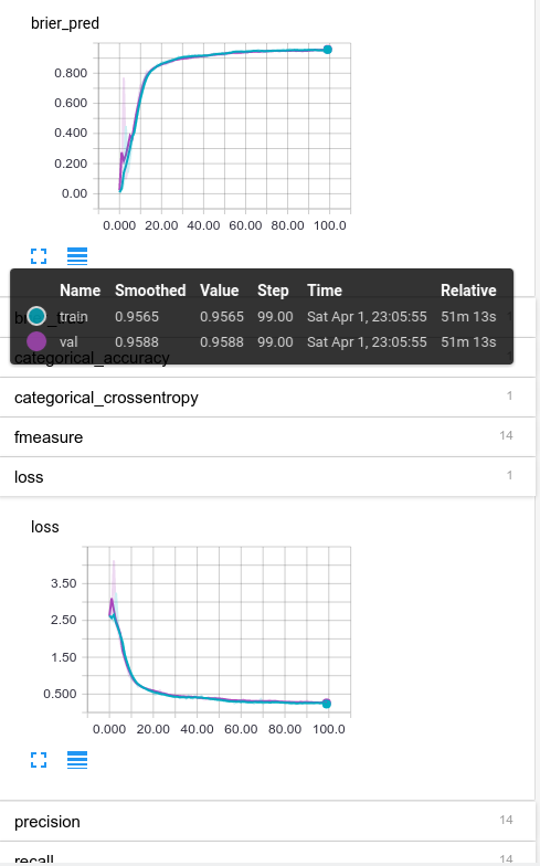
Tensorboard view of training and validation results
I’ve expanded the brier_pred plot and the loss (which is categorical crossentropy in this case) so we could see the performance curve. The main thing to notice is that the training (blue) and validation (purple) curves are right on top of each other, indicating we aren’t overfitting. So that’s good.
We also see that the shape of brier_pred and loss are similar; meaning the algorithms self-confidence (brier_pred only looks at the predicted probabilities and not actual ones) matches the real ones reasonably well. Also good.
Finally, take a look at the performance mousover states. The final Brier scores are ~0.96, not half-bad!
Also notice that there are 14 quantities being tracked under fmeasure, precision, and recall. These correspond to the “binary” metrics for our 14 classes. If you’re following along at home, you should be able to expand those and view line plots for each of the 14 classes individually; for example here are the fmeasure plots for 6 classes:
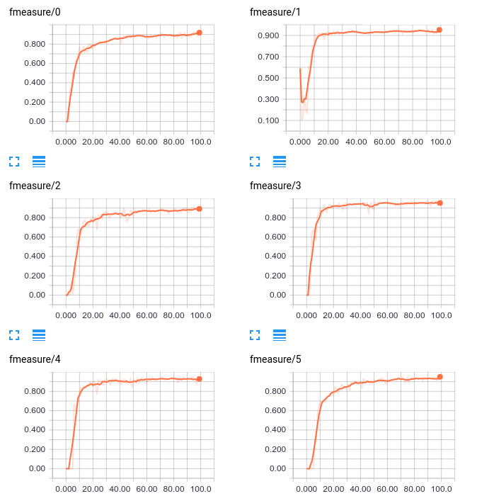
F-Measure on Validation set for first six classes
We see that most classes start roughly at 0, except class 1 where it starts close to 0.5. F-Measure is the harmonic mean of precision and recall, presumably a starting point is just predicting everything as one class. As the model learns, the performance becomes more even.
We can also look at these statistics in histogram form:
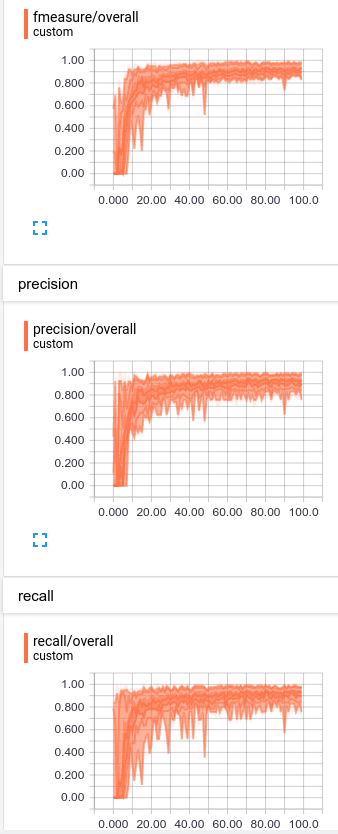
Histogram of binary metrics
Performance on each statistic varies from 0.8 – 1.0, so we aren’t wildly off-base on any particular class.
Comparing Models
Now we can tweak some model parameters and see how the performance (both runtime and accuracy) vary. We test out three models:
- Pick our own vocabulary and train embeddings based on the dataset
- Pre-specified word embeddings and vocabulary, and also allow additional training of the word embeddings. Jumping off the shoulders of giants, as it were.
- Default configuration. Pre-specified word embeddings and vocabulary
| Model 1 (De novo) | Model 2 (Pre-specified but trainable) | Model 3 (fully pre-specified) | |
|---|---|---|---|
| Training Time (hh:mm:ss) | 0:54:26 | 54:25 | 51:59 |
| Validation Loss | 0.2326 | 0.1733 | 0.2625 |
| Validation Accuracy (Chance: 7.14%) | 92.90% | 94.50% | 91.90% |
| Validation Time (sec) | 6.86 | 6.72 | 7.07 |
We see that Model 2 has the best performance, although the differences are slight. Intuitively this is to be expected; the pre-trained vectors make use of an enormous corpus of text, but it can still be fine-tuned for this purpose. Model 3 is the fastest to train, since it has the fewest free parameters, and still achieves good performance.
Conclusion
We have learned how to log both the inputs of a model (Sacred could be used for any computational experiment btw, not just machine learning) and some hacks which can improve logging using Keras and Tensorflow. This post has largely showcased the downside of using a library like Keras. While it makes some things extremely easy, anything out of its scope becomes much harder.
Next time we’ll do something a little bit more interesting, and look at methods of visualizing the textual content itself. Stay tuned!
-Jacob
- [1]https://en.wikipedia.org/wiki/Brier_score↩
- [2]Pablo Tamayo, Daniel Scanfeld, Benjamin L. Ebert, Michael A. Gillette, Charles W. M. Roberts, and Jill P. Mesirov
Metagene projection for cross-platform, cross-species characterization of global transcriptional states
PNAS 2007 104 (14) 5959-5964; published ahead of print March 27, 2007, doi:10.1073/pnas.0701068104
http://www.pnas.org/content/104/14/5959.abstract↩ - [3]https://en.wikipedia.org/wiki/Precision_and_recall↩
- [4]Keras is under the MIT license so this is fully permitted↩
- [5]Do feel free to email or comment with others↩

Its very informative article. Thanks for sharing with us.
Actually I am trying to log precision, recall fmesure for multi-label image classification. I used code for custom_metrics that you mentioned here but my model is not storing any log inside custom_directory. Do I have to do anything else accept calling : create_batch_pairwise_metrics(y_true, y_pred)
in my model?
Make sure you have the custom tensorboard saver as a callback
Thanks for your reply. I am using custom tensorboard saver as callback. Directory for custom has been created but no log file inside it.